Gridiron Skew Part 1

Something you have already guessed: your humble blogger is a bit of a nerd. And, I really nerd out on football. It is a great sporting frontier of obstinate complexity. Twenty-two men with different, overlapping and constantly fluctuating jobs operate from a multitude of formations on a field that, conceptually, is massive, continental, vast. This is no pitcher-vs-batter game, is not even as simple as basketball. Football is to other sports as chess is to checkers.

So naturally, it's exciting to an amateur mathnerd like myself to see that folks out there on the intertubes are trying to make sense of the pile of data generated by each single football game. Granted, some of this is of the "We calculate this metric from a privileged position" variety, or baldly dismissive of core mathematical concepts¹. But Chris Brown of Smart Football really digs up some gems, and he's more than willing to tantalize us with his methods. He talks about game theory and its application to run/pass balance. He mentions the Sharpe ratio when evaluating the effectiveness of a play. Every step wrings a little more heuristics out of the great game. This, my friends, is awesome.

For instance, the aforementioned Sharpe ratio. As Chris puts it:

The Sharpe Ratio is defined as the ratio of the difference between the expected return of some strategy minus the expected return of some riskless benchmark and the standard deviation of the strategy.

[ed: This can be written as such for those of us who like equations]

Standard deviation is a measurement of the volatility of a set of values. You can read more about standard deviation here. For example, if a given pass play was run four times, and the results (in yards) of the play was 10, 10, 10, and 10, it has a standard deviation of 0. However, if it was run four times and the results were 0, 0, 40, and 0, it has the same average gain (10 yards) but its standard deviation would be 20. We would prefer pass play one to pass play two. It has the same expected gain, but it is less risky than the second.

This is all well and good. What's more, the Sharpe ratio may be used to determine the ratio with which you use one strategy (or one play) over another. If one play's Sharpe ratio is 2 and the other play's Sharpe ratio is 4, you should use the latter play twice as often as the former. The power of this method is clear when you begin sectioning your data ever more finely - the Sharpe ratio allows us to compare any number of situations. How do your different running plays fare on second down and less than five yards? Out of which formation is play-action most effective? At what position on the field is your offense most able to run the HB draw to the near side out of a pro set in the fourth quarter on third down with more than four yards to go? With enough data, the Sharpe ratio can help you answer that question.

However, the Sharpe ratio is weak in a critical aspect: it punishes inconsistency. Why is that a weakness? Take, for example, the first pass play postulated: absolute, robotic 10 yards per attempt. Sounds like a great play. What could be better, though, is a play that results in a 20 yard gain every fourth attempt (10, 10, 10, 20.) It's clear to everyone and their blind, demented uncle that 10, 10, 10, 20 is better than 10, 10, 10, 10. And yet, the Sharpe ratio is misleading. Because we divide by standard deviation, a play's inconsistency - whether the play succeeds wildly or fails miserably - is punished. Essentially, when you calculate the Sharpe ratio, you are implicitly assuming that an offensive big play and a defensive big play are equally horrible. This weakness becomes especially clear when one starts adjusting yardage totals for touchdowns and turnovers. A helpful guy out on the interwebs has run the calculations: a touchdown or a turnover is basically equivalent to 50 yards. But if your goal line play wins you a touchdown every fourth attempt - certainly an effective play - that's 1, 1, 1, and 51. Standard deviation is so high that it will obliterate your statistical decision-making.

I'm picking on the Sharpe ratio because its promises are so tantalizing, and yet I think it asks the wrong question. What we should be ascertaining is the level of skew in the yards gained by each play. Aside perhaps from Jim Tressel, coaches value big-play capability just as much as they dread the defense's ability to ram a big play down their throat. We all want our teams to be explosive. Just, explosive in the downfield direction. To put it in the terms of the shape of a distribution, we want the yards-per-play distribution to have a negative skew, like so (via): Skew answers the question, does a play regularly succeed? If there is negative skew, the answer is yes. So how do we reward negative skew in our analyses?

I should probably put the rest in another post...




1. Direct quote:

I do agree ... that R-squared gives you "the proportion of variance that is in common between NBA team payroll and NBA team performance." But what does that mean? Almost nothing, unless you're a statistician.

Similarly, one could declare that "I do agree that USC hammered the seams in Penn State's overmatched cover 3 defense, but what does that mean? Almost nothing, unless you're talking about football." May as well come out and say "I don't understand how to use this metric but I'm going to criticize it."

Monopoly Properties

Edit: WIFE! WIFE! WIFE!

Recently, I was playing Monopoly with my darling wife. The first game, I got lucky and bought all four railroads and the orange set of properties. I leveraged everything for hotels and won that game handily. But the second game brought the nightmare scenario: all properties purchased, no monopolies.

Rather than restart the game, we began bargaining. I resolved to hold firm until I got a deal that favored my cause - don't look at me like that, she's more competitive than I - and rejected a couple of her trades right off the bat. But then, she offered me one I couldn't pass up. I had two out of three green squares (heretofore my favorite properties) and two out of three red squares. She had two out of three yellow squares. Her proposal: trade her the last yellow property and one of the reds for the last green. I eagerly accepted, again mortgaged everything to buy houses... and got completely hosed. I looked at her yellow properties - three hotels - and looked at my greens, with three or four houses apiece. Needless to say, successfully running that gauntlet was never going to happen.Now this was remarkable - the orange properties clearly annihilated the a block of properties three full blocks ahead of them. Clearly, there was some hidden pattern that one could exploit in a trade. Of course, my nerd-sense was piqued. "I can feel an Excel spreadsheet coming on..." I said. She just shook her head.


BTW: I'm just a single nerd. Any nerds who want to CMIIW, well, I'll buy you a Coke.


Here's the board in question:


Property cost increases in a fairly continuous manner as one travels around the board. If we exclude the purples and the dark blues, cost of property begins at $100 and increases by $20 every time the last or first property in a block is reached. Likewise, house cost increases stepwise by $50, with the first flight of properties requiring $50 per house, the second requiring $100, the third requiring $150, and the fourth requiring $200.



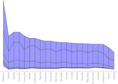
Taking them together, we can plot the cost of attaining the different states (0 houses, 1 house, 2 houses...) for each property:



One can already see that the two twin-property blocks (purples and dark blues) don't fit the trend - they are simply too cheap to develop because you only have to buy two of them to start building houses. This is obvious, of course. What I hadn't expected was that price would peak at the green properties - Boardwalk and Park Place require a slightly larger initial investment per-property, but are still cheaper to develop than their preceding neighbors. The green properties are the most expensive to develop on the entire board.

Rent increases in a continuous yet idiosyncratic manner:



Trends are less illuminating here. We notice the gradual increase from left-to-right, and the fact that no single property charges less rent than any property before it. But other than that, there doesn't seem to be any unifying trend. The behavior in the mauve block is particularly weird, and again, the twin-property blocks are outliers.


But how do those trends interact? Monopoly's nut and bolts are proper investment - therefore, one should form a trading strategy that maximizes return on investment. Of course it's true that merely breaking even on a property does not mean you've bankrupted your opponent. However, breaking even does mean that you've spent less money on that property than your opponent - the soul of good development. So I figured one could roughly model a property's success rate by calculating the probability that the greedy landlord will recoup their initial ante.

First, we must calculate the ratio of rent to investment. For a single, naked property, that would be the rent you collect divided by the purchase cost of that property:

and for a property with houses:

This number shows us how much money one gets in rent as a percentage of the money you invested into the property - the efficiency of investment. I calculated this number for all states of the property (zero houses, one house, two houses, etc.):



A visually-pleasing color-coded version, you say? Voila:



Another trend becomes evident: the first block of properties in a flight is less efficient than the second block. You pay the same for a house in the red block as you do in the yellow block, but you get less rent out of it. Thus, while no property charges less rent than any property before it, some properties charge less rent per dollar invested than some properties before them. IE, they have a lower . Also, it's important to see that the first half of the board already seems much more efficient than the second half, per-land. This is pretty critical. And lastly, it is interesting to note that efficiency has an S-curve, reaching a peak derivative at the third stage of property development. increases slightly on adding the first house, moreso with the second house, increases the most dramatically with the third house, and there are diminishing returns from then on.

From we can calculate the number of times the property must be landed upon in order to fully recoup the investment:

Pretty simple. The number of times one must land on the property is the number of times that the rent goes into the investment:



This number is useful when we consider the probability of landing on each property. It is conceivably possible to calculate the probability of landing on each property based on its position - I don't know how to do that. Lucky for us, a helpful guy out on the interwebs has done just that:



Note: he's approached the game differently than I. Take that as you will.

He has determined the probabilities based on two different game strategies. The "short" strategy is an early-game strategy in which players pay to get out of jail as quickly as possible, so to buy up property. The "long" strategy is a late-game strategy in which players stay in jail as long as possible, so to avoid paying rent. This strategy increases the probability of being in jail a little less than three-fold, which we would expect - players may stay in jail until they pay, roll doubles, or three turns have passed at which time they must pay $50 and leave. For the regular properties, this means the probability of landing on any property space is somewhat decreased. There are some weirdnesses associated with that, but I'm really not qualified to discuss them.

First, notice the random peaks at Illinois, New York, Boardwalk, and St. Charles. You can be sent to all three of these properties directly by chance cards. New York is a lesser peak because its card is "Go Back Three Spaces" which has different effects based on which of three chance locations you have landed on. You can also be sent to Go, Reading Railroad, or to Jail by cards (or by the Go To Jail square.) All of this tends to weight the front half of the board much more heavily in terms of probability. Essentially, the probability peaks around free parking (though this doesn't explain why I never land on free parking and my wife always does. Go figure.) This shows us that while the earlier properties may not draw as much rent, you do land on them more often.

So how do those two trends (required lands and probability of a single land) interact? Now that we know the probability of landing on each square and we know the required number of landings to recoup investment, it is simple to calculate the probability of breaking even. If a certain event has a probability A, the probability of that event occurring B number of times is A^B. So, the probability of recouping an investment in a single Monopoly property by landing only on that property is:

A graph of that is pretty interesting. Here are two graphs, for "short" and "long" strategies respectively:




First off, I know what everyone is already thinking: Park Place/Boardwalk appear bizarrely awesome, total outliers. Likewise, Mediterranean Avenue and Baltic Avenue appear absolutely worthless. Within the middle eighteen properties, where a strong trading strategy is less immediately intuitive, the function clearly points to a sweet spot around the mauve properties. In particular, it points to the light blue properties - somewhat of a surprise. If Monopoly was the Houston Rockets, then Connecticut Avenue would appear to be Shane Battier.


But that still doesn't tell us everything. After all, one does not buy single properties in Monopoly. One buys streets, the success of which is dependent upon the success of all two or three properties therein. Calculating the successfulness of each block is a little trickier. If you're a math geek and I've made an error somewhere, step in. Here's my approach. What we need first is the rent which we are likely to be charged if we land within a certain block. This is not the simple arithmetic mean of the rents being charged on all three properties. If Baltic charges $1,000 and Mediterranean charges $1, the arithmetic mean is $500.50. But if Baltic gets a land 1% of the time and Mediterranean gets the remaining 99%, the true likely rent value is much closer to $1. We really need to model the land as two events: landing on a certain block, and landing on a particular square within the block. The process is akin to a current divider, or partial pressures in chemistry. If a player lands within a certain block, the probability he will land on a certain square is the independent probability of landing on that square divided by the probability of landing on any square in that block (the sum of the probabilities.) We can then multiply the resultant probabilities by their corresponding rents, and add these together to get a probability-adjusted rent for the entire block:

= probability of landing on a particular property (n) in the block
= probability of landing on one of those properties (IE, sum of the probabilities)
= the rent charged by that property (n) with a certain number of houses (h)

And the graph thereof:



Note: in this calculation I've assumed that all three properties would have the same number of houses. I may have some time on my hands, but I don't have the kind of time I'd need to calculate all 4,032 combinations.

Investment, likewise, was calculated by summing the costs of all three properties, plus the cost of all the houses:



Rent/investment ratio is calculated as before, but with the adjusted values:



And of course, the charismatic colored version:



And again we graph the reciprocal, which shows us the number of lands necessary to recoup investment. Nothing new here, there is an abrupt dip at the orange block:



Broadway's grip is slowly weakening...

For the calculation of whole-block probabilites, the value used for probability is the sum of the probabilities of the squares within each block. Compared to the earlier graph of probability (which is somewhat of a mess) this one is exceedingly clear. Probability peaks somewhere around free parking:



Using these recalculated values, probability of recouping investment is calculated as before

...giving us this graph:




And it's rather profound. The orange properties are easily the best on the board - even better than the vaunted Broadway and Park Place. And my beloved green properties? Nasty, nasty bad. The maximum probability of recouping your investment on the greens is 0.0004, or 1 in 2500. Comparatively, the maximum for the orange properties is 0.05, or 1 in 20. This does not mean that buying and developing the orange properties will bankrupt your opponent automatically - the greens obviously have more "killing power" per land. However, they get landed upon so infrequently and are so expensive to develop, you hurt yourself far more than your opponent.

The Airplane on a Treadmill

The problem is as follows:

Suppose that there is an airplane on a treadmill, a treadmill as long and wide as a runway. The treadmill is designed such that its speed exactly matches the speed of the airplane's wheels, but moving in the opposite direction. Can the plane take off?

It's a neat question, if only for the visual of a 747 on a treadmill, its turboprops amounting to the world's largest hair dryers as the treadmill hums underneath madly spinning landing gear. And it's certainly true that a treadmill could push a plane backwards hard enough that it could fully oppose the thrust from the plane's engines.

Typical approaches toward this problem have been mathematical and focused on defining the velocity of the treadmill itself. However, I don't think that's the right tack. The question is deceptively formulated and conceals the issue at the heart of this problem: not velocity, but acceleration. We can assume that the plane has a velocity below escape velocity, else it would already be airborne. Moreover, whether it begins at 0mph or somewhere in the middle isn't important in principle - the goal of the plane, whatever its initial velocity, is to accelerate to the velocity at which its wheels leave the green earth. The goal of the treadmill, therefore, is to prevent any acceleration, as with a non-zero acceleration the plane will eventually reach escape velocity. Or more realistically, with a non-zero acceleration the question turns into an engineering problem: are the plane's engines strong enough to accelerate it quickly enough to reach escape velocity, even when opposed by the treadmill?¹

So, the question becomes: can the treadmill prevent the plane from accelerating, by adjusting to the plane's velocity?

And the answer is no, it can't. In order for the treadmill to prevent the plane's speed from changing, the treadmill must be able to speed up itself. But the treadmill's speed is tied directly to the plane's wheels speed. Therefore, in order to speed up it must detect a change in the plane's velocity. IE, in order for the treadmill to speed up, the plane itself must first speed up. The plane has therefore a non-zero acceleration, and eventually takes off. Moreover, the treadmill can't keep the plane from accelerating even by adjusting for the plane's acceleration, for it would not be able to prevent a change in acceleration, or, jerk. You could keep rolling down that chain of derivatives forever, becoming perhaps more efficient but never truly keeping that plane on the ground. This is because these systems - adjusting for impulse change in velocity and adjusting for impulse change in acceleration - are identical in concept. An impulse change in velocity is a discontinuous function, which means that not only would you change the function itself, but you change all of its derivatives. Therefore, speed, acceleration, jerk, etc. are all the same thing here. And given a long enough treadmill (or a short enough treadmill ¹) the plane can not be prevented from accelerating. Its acceleration may only be incompletely opposed.

The issue at the heart is that one can not prevent change by reacting to change, and one can not negate change by correcting to the change instead of correcting for the change. I could put it to you another way: suppose that the devil has a glass of ice water he wants to save for dinner, and he charges one of his demons to keep the ice from melting. The demon, being a little behind the curve, puts the ice water in the freezer whenever he sees some ice melt, but fearing the devil's wrath should the glass of water freeze solid, he removes the glass shortly after putting it in. He's a very fast demon, perhaps, and reacts quickly to the smallest melting. But the demon's task is impossible, for the change he is trying to prevent is a change he may only react to, and not a change he can correct for.

The only way to hold the plane down would be to adjust the treadmill's speed (and thereby, the acceleration due to the frictional force on the landing gear) in concert with the thrust produced by the plane's engines. But then the question - if a plane's thrusters are perfectly opposed by some other force, can it take off? - is really dumb.


Hat tip to the XCKD blag, which gave me this idea and that awesome picture in the first place.




1 Actually, if the plane accelerates at all it will eventually leave the treadmill. Since the treadmill is of finite length (as long and wide as a runway,) if the plane moves at all with respect to the treadmill it's good as in the sky. Well, unless the treadmill was constructed at LaGuardia.